Get Started

This page contains basic usage of dte_adj library.

Generate data for training cumulative distribution function:

import numpy as np

def generate_data(n, d_x=100, rho=0.5):
    """
    Generate data according to the described data generating process (DGP).

    Args:
    n (int): Number of samples.
    d_x (int): Number of covariates. Default is 100.
    rho (float): Success probability for the Bernoulli distribution. Default is 0.5.

    Returns:
    X (np.ndarray): Covariates matrix of shape (n, d_x).
    D (np.ndarray): Treatment variable array of shape (n,).
    Y (np.ndarray): Outcome variable array of shape (n,).
    """
    # Generate covariates X from a uniform distribution on (0, 1)
    X = np.random.uniform(0, 1, (n, d_x))

    # Generate treatment variable D from a Bernoulli distribution with success probability rho
    D = np.random.binomial(1, rho, n)

    # Define beta_j and gamma_j according to the problem statement
    beta = np.zeros(d_x)
    gamma = np.zeros(d_x)

    # Set the first 50 values of beta and gamma to 1
    beta[:50] = 1
    gamma[:50] = 1

    # Compute the outcome Y
    U = np.random.normal(0, 1, n)  # Error term
    linear_term = np.dot(X, beta)
    quadratic_term = np.dot(X**2, gamma)

    # Outcome equation
    Y = 5 * D + linear_term + quadratic_term + U

    return X, D, Y

n = 1000  # Sample size
X, D, Y = generate_data(n)

Then, let’s build an empirical cumulative distribution function (CDF).

import dte_adj
from dte_adj.plot import plot

estimator = dte_adj.SimpleDistributionEstimator()
estimator.fit(X, D, Y)
locations = np.linspace(Y.min(), Y.max(), 20)
cdf = estimator.predict(1, locations)

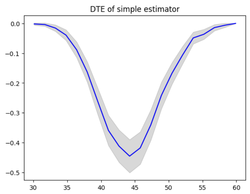
Distributional treatment effect (DTE) can be computed easily in the following code.

dte, lower_bound, upper_bound = estimator.predict_dte(target_treatment_arm=1, control_treatment_arm=0, locations=locations, variance_type="simple")

A convenience function is available to visualize distribution effects. This method can be used for other distribution parameters including Probability Treatment Effect (PTE) and Quantile Treatment Effect (QTE).

plot(locations, dte, lower_bound, upper_bound, title="DTE of simple estimator")

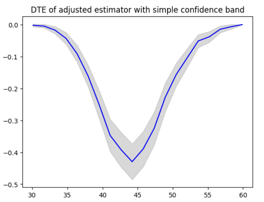
To initialize the adjusted distribution function, the base model for conditional distribution function needs to be passed. In the following example, Logistic Regression is used. Please make sure that your base model implements fit and predict_proba methods.

from sklearn.linear_model import LogisticRegression
logit = LogisticRegression()
estimator = dte_adj.AdjustedDistributionEstimator(logit, folds=3)
estimator.fit(X, D, Y)
cdf = estimator.predict(1, locations)

DTE can be computed and visualized in the following code.

dte, lower_bound, upper_bound = estimator.predict_dte(target_treatment_arm=1, control_treatment_arm=0, locations=locations, variance_type="simple")
plot(locations, dte, lower_bound, upper_bound, title="DTE of adjusted estimator with simple confidence band")

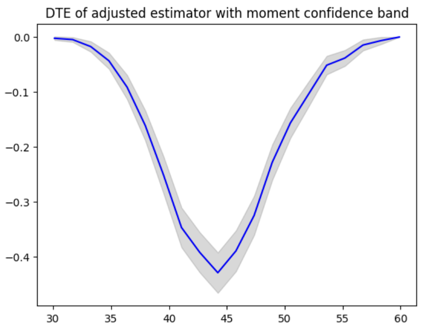
Confidence bands can be computed in different ways. In the following code, moment condition is used to calculate the confidence band.

dte, lower_bound, upper_bound = estimator.predict_dte(target_treatment_arm=1, control_treatment_arm=0, locations=locations, variance_type="moment")
plot(locations, dte, lower_bound, upper_bound, title="DTE of adjusted estimator with moment confidence band")

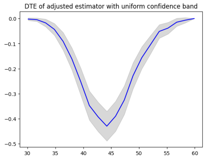
Also, an uniform confidence band is used when uniform is specified for the variance_type argument.

dte, lower_bound, upper_bound = estimator.predict_dte(target_treatment_arm=1, control_treatment_arm=0, locations=locations, variance_type="uniform")
plot(locations, dte, lower_bound, upper_bound, title="DTE of adjusted estimator with uniform confidence band")

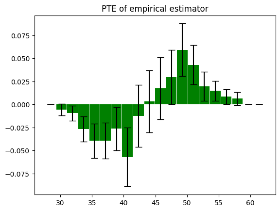
To compute PTE, you can use predict_pte method. The locations parameter defines interval boundaries, and the method returns probability treatment effects for each interval. For each interval, the starting point is not included but the ending point is included. For example, if the locations is [0, 1, 2], PTE is computed for (0, 1] and (1, 2].

pte, lower_bound, upper_bound = estimator.predict_pte(target_treatment_arm=1, control_treatment_arm=0, locations=locations, variance_type="simple")
# Note: pte will have shape (len(locations)-1,) since it computes intervals between locations
plot(locations[:-1], pte, lower_bound, upper_bound, chart_type="bar", title="PTE of adjusted estimator with simple confidence band")

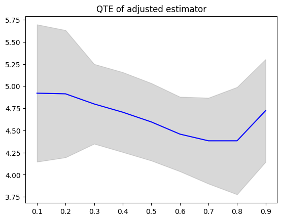
To compute QTE, you can use predict_qte method. The confidence band is computed by bootstrap method.

quantiles = np.array([0.1 * i for i in range(1, 10)], dtype=np.float32)
qte, lower_bound, upper_bound = estimator.predict_qte(target_treatment_arm=1, control_treatment_arm=0, quantiles=quantiles, n_bootstrap=30)
plot(quantiles, qte, lower_bound, upper_bound, title="QTE of adjusted estimator")

You can use any model with predict_proba or predict method to adjust the distribution function estimation. For example, the following code use XGBoost classifier to estimate the conditional distribution.

import xgboost as xgb
estimator = dte_adj.AdjustedDistributionEstimator(xgb.XGBClassifier(), folds=3)
estimator.fit(X, D, Y)
cdf = estimator.predict(1, locations)

predict_dte and predict_pte methods provide an option to train a model for multiple locations simultaneously. To enable the feature, pass is_multi_task=True.

from sklearn.linear_model import LinearRegression
model = LinearRegression()
estimator = dte_adj.AdjustedDistributionEstimator(model, folds=3)
estimator.fit(X, D, Y)
dte, lower_bound, upper_bound = estimator.predict_dte(target_treatment_arm=1, control_treatment_arm=0, is_multi_task=True, locations=locations, variance_type="moment")